Wavefunction#
This example shows a minimal Python workflow for wavefunctions in an atomic-orbital(AO) basis.
Recall that the real-space Bloch wavefunction and the AO wavefunction are related by
and the periodic part of the Bloch wavefunction and the AO wavefunction are related by
here \(\phi_{j\beta}\) are the basis functions, and \(c_{n, j\beta}(\boldsymbol{k})\) are the AO wavefunction coefficients.
Starting from a DeepH data point containing hamiltonian.h5, overlap.h5, POSCAR, and info.json, we will:
diagonalize the generalized eigenvalue problem \(H(k)c = E S(k)c\) at the Gamma point,
save the AO wavefunction coefficients to
wavefunction_ao.h5, anduse
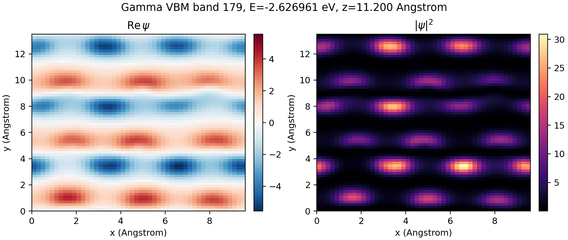
AOWfnObjto evaluate and plot the Gamma-point highest valence-band wavefunction in real space. (currently only supports SIESTA and OpenMX.)
Setup#
import os
from pathlib import Path

# Use writable cache directories on shared systems.
os.environ.setdefault("MPLCONFIGDIR", "/tmp/deepx_dock_matplotlib")
os.environ.setdefault("XDG_CACHE_HOME", "/tmp/deepx_dock_cache")
os.environ.setdefault("MPICH_GPU_SUPPORT_ENABLED", "0")
import h5py
import matplotlib.pyplot as plt
import numpy as np

from deepx_dock.CONSTANT import DEEPX_WFNAO_FILENAME
from deepx_dock.compute.eigen.hamiltonian import HamiltonianObj
from deepx_dock.compute.eigen.wavefunction import AOWfnObj

DATA_ROOT = Path("wavefunction.clean/BLBP")
DATA_DIR = DATA_ROOT / "0"
BASIS_DIR = DATA_ROOT / "basis"
FIG_DIR = Path("figures.bak")
FIG_DIR.mkdir(exist_ok=True)

E_FERMI_EV = -2.4558
KPTS = np.array([[0.0, 0.0, 0.0]])
# Real-space grid used only for this small plotting example.
GRID = np.array([48, 68, 100])
1. Diagonalize the Hamiltonian#
HamiltonianObj loads both hamiltonian.h5 and overlap.h5. Calling diag(..., bands_only=False) solves the non-orthogonal generalized eigenvalue problem and returns both energies and eigenvectors.
eigvalshas shape(n_band, n_k).eigvecshas shape(n_orb, n_band, n_k).
ham = HamiltonianObj(DATA_DIR)

eigvals, eigvecs = ham.diag(
    KPTS,
    n_jobs=1,
    parallel_k=True,
    bands_only=False,
)

gamma_eigs = eigvals[:, 0]
occupied = np.flatnonzero(gamma_eigs <= E_FERMI_EV)
if len(occupied) == 0:
    raise RuntimeError(f"No occupied band found below E_FERMI_EV={E_FERMI_EV}")

vbm = int(occupied[-1])
cbm = vbm + 1

print(f"Number of orbitals: {ham.orbits_quantity}")
print(f"Eigenvalues shape: {eigvals.shape}")
print(f"Eigenvectors shape: {eigvecs.shape}")
print(f"Gamma VBM band index: {vbm}")
print(f"Gamma VBM energy: {gamma_eigs[vbm]:.12f} eV")
print(f"Gamma CBM band index: {cbm}")
print(f"Gamma CBM energy: {gamma_eigs[cbm]:.12f} eV")
Number of orbitals: 1584
Eigenvalues shape: (1584, 1)
Eigenvectors shape: (1584, 1584, 1)
Gamma VBM band index: 179
Gamma VBM energy: -2.626961019206 eV
Gamma CBM band index: 180
Gamma CBM energy: -2.186534744865 eV
Diagonalizing:   0%|          | 0/1 [00:00<?, ?it/s]
Diagonalizing: 100%|##########| 1/1 [00:06<00:00,  6.29s/it]
Diagonalizing: 100%|##########| 1/1 [00:06<00:00,  6.30s/it]
2. Save AO wavefunction coefficients#
AOWfnObj.load expects AO coefficients with shape (n_k, n_band, n_orb). The eigenvectors returned by HamiltonianObj.diag are (n_orb, n_band, n_k), so we transpose them before loading.
After loading, AOWfnObj.to_h5() writes wavefunction_ao.h5 in the data directory by default.
wfn = AOWfnObj(DATA_DIR, BASIS_DIR, "siesta")

# Convert (n_orb, n_band, n_k) -> (n_k, n_band, n_orb).
wfnao = eigvecs.transpose(2, 1, 0)

wfn.load(
    KPTS,
    wfnao,
    eigvals.T,
    spinful=False,
    efermi=E_FERMI_EV,
    kgrid=(1, 1, 1),
)

wfn.to_h5()
wfnao_path = DATA_DIR / DEEPX_WFNAO_FILENAME

print(f"Saved AO wavefunction coefficients to: {wfnao_path}")
with h5py.File(wfnao_path, "r") as h5f:
    print("Saved datasets:", sorted(h5f.keys()))
    print("eigenvectors shape:", h5f["eigenvectors"].shape)
Saved AO wavefunction coefficients to: wavefunction.clean/BLBP/0/wavefunction_ao.h5
Saved datasets: ['efermi', 'eigenvalues', 'eigenvectors', 'kgrid', 'kpts']
eigenvectors shape: (1, 1584, 1, 1584)
3. Compute and plot the real-space wavefunction#
AOWfnObj.to_real_space evaluates the selected AO wavefunction on a uniform real-space grid. Here we evaluate only the Gamma-point highest valence band.
If the wavefunction is evaluated on a real space grid of size \(n_x \times n_y \times n_z\), the real-space wavefunction is normalized to \(\sqrt{n_x n_y n_z}\).
# psi shape: (selected_n_k, selected_n_band, n_spinor, nx, ny, nz).
psi = wfn.to_real_space(
    ik=0,
    ib=vbm,
    gridsize=GRID,
    return_periodic=True,
)

psi_vbm = psi[0, 0, 0]
norm = np.sum(np.abs(psi_vbm) ** 2)

print(f"Real-space wavefunction shape: {psi.shape}")
print(f"Norm: {norm/np.prod(GRID):.12f}")
Real-space wavefunction shape: (1, 1, 1, 48, 68, 100)
Norm: 1.000010331947
# Use the z slice with the largest integrated density for a readable 2D image.
density = np.abs(psi_vbm) ** 2
z_slice = int(np.argmax(density.sum(axis=(0, 1))))
fig, axes = plt.subplots(1, 2, figsize=(9, 3.8), constrained_layout=True)

real_slice = psi_vbm[:, :, z_slice].real.T
density_slice = density[:, :, z_slice].T

# Convert grid indices to real lengths along lattice vectors a, b, and c.
cell_lengths = np.linalg.norm(ham.lattice, axis=1)
extent_xy = [0.0, cell_lengths[0], 0.0, cell_lengths[1]]
z_coord = z_slice / GRID[2] * cell_lengths[2]

real_limit = float(np.max(np.abs(real_slice)))
im = axes[0].imshow(
    real_slice,
    origin="lower",
    cmap="RdBu_r",
    vmin=-real_limit,
    vmax=real_limit,
    aspect="auto",
    extent=extent_xy,
)
axes[0].set_title(r"$\mathrm{Re}\,\psi$")
axes[0].set_xlabel("x (Angstrom)")
axes[0].set_ylabel("y (Angstrom)")
fig.colorbar(im, ax=axes[0], fraction=0.046, pad=0.04)

im = axes[1].imshow(
    density_slice,
    origin="lower",
    cmap="magma",
    aspect="auto",
    extent=extent_xy,
)
axes[1].set_title(r"$|\psi|^2$")
axes[1].set_xlabel("x (Angstrom)")
axes[1].set_ylabel("y (Angstrom)")
fig.colorbar(im, ax=axes[1], fraction=0.046, pad=0.04)

plot_path = FIG_DIR / "vbm.png"
fig.suptitle(f"Gamma VBM band {vbm}, E={gamma_eigs[vbm]:.6f} eV, z={z_coord:.3f} Angstrom")
fig.savefig(plot_path, dpi=220)

plt.show()