Hamiltonian Diagonalization#
The Hamiltonian itself is not a physical observable, but its eigenvalues (i.e., energy levels) are. To get the eigenvalues of a Hamiltonian for a periodic crystal, it is convenient to transform the Hamiltonian into reciprocal space (Brillouin zone) labeled by \(k\), and the Hamiltonians on different \(k\) points are decoupled from each other.
A periodic Hamiltonian: \(H_{ij,R_1,R_2}=H_{ij,0,R_2-R_1}\doteq H_{ij,R_2-R_1} \ \ \ \ \forall R_1,R_2\)
Fourier transform: \(H_{ij(k)}=\sum_R e^{\mathbb{i}kR}H_{ij,R}\)
A generalized eigenvalue problem \(H_{(k)} |\psi_{k}\rangle = \varepsilon_{(k)} S_{(k)} |\psi_{k}\rangle\) can be solved on each \(k\) point seperately. The eigenvalues \(\varepsilon_{(k)}\) form the electronic band structure (band energies).
DeepH-dock provides a set of diagonalization interfaces which take the DeepH-pack format data as input, construct the Hamiltonian matrix, and invoke scipy.linalg.eigh to diagonalize the Hamiltonian.
Fermi energy#
The fermi energy \(\varepsilon_F\) is defined as the energy level where the number of states below is equal to the electronic occupation.
where \(D_{(\varepsilon)}\) is density of states and \(N_{\text{ele}}\) is electronic occupation. The number of states below an energy level can be directly counted out or integrated out using the tetrahedron method.
To determine the fermi energy via the tool in DeepH-dock, the occupation number should be added to the info.json file. Note that the occupation always includes the spin degree of freedom, even when spinful is set to false.
{
  "occupation": 46,
  ...
}
The fermi energy can be determined by the command below.
dock compute eigen find-fermi -h
Usage: dock compute eigen find-fermi [OPTIONS] DATA_PATH

  Find the Fermi energy using the number of occupied electrons.

Options:
  -j, --jobs-num INTEGER          Number of parallel workers. Default: -1 (auto-detect CPU cores).  [default: -1]
  --blas-parallel-mode            Use BLAS multi-threaded mode instead of parallel k-point mode (default).
  --method [counting|tetrahedron]
                                  Calculating method that is used for obtaining DOS.  [default: counting]
  -d, --kp-density FLOAT          The density of the k points.  [default: 0.1]
  --cache-res                     Cache the eigenvalues so that you can save time in the subsequent DOS calculation.
  --ill-method [none|window|orbital]
                                  Method to handle ill-conditioned eigenvalues.  [default: none]
  --ill-threshold FLOAT           Threshold for ill-conditioned eigenvalue detection.  [default: 0.001]
  --window-emin FLOAT             Minimum energy for window regularization (eV, relative to Fermi).  [default: -1000.0]
  --window-emax FLOAT             Maximum energy for window regularization (eV, relative to Fermi).  [default: 6.0]
  -h, --help                      Show this message and exit.
The calculation directory DATA_PATH should contain POSCAR, info.json, overlap.h5, and hamiltonian.h5. A 3D mesh of \(k\) points is generated based on the three reciprocal lattice vectors, and the \(k\) point spacing is determined by kp-density (measured in \(\text{Ang}^{-1}\)).
Parallelization Strategy:
Default (without
--blas-parallel-mode): Multiple k-points processed in parallel, each using single-threaded BLAS. Best for many small k-point calculations.With
--blas-parallel-mode: K-points processed sequentially, each using multi-threaded BLAS. Best for few large matrix diagonalizations.
The default method for the integration of \(D_{(\varepsilon)}\) is counting the number of energy levels, which is convenient for insulators but inaccurate for metals. One can switch to the tetrahedron method by setting --method tetrahedron to perform more accurate calculation, which invokes the libtetrabz package. The eigenvalues will be dumped if --cache_res is specified and can be used to plot the density of states (see the next section). After the calculation, a file named fermi_energy.json is dumped. If needed, the fermi energy stored in the fermi_energy.json can replace the one in info.json.
Example:
dock compute eigen find-fermi ./eigen/MoTe2 -d 0.1 -j 16
Use dk=0.1 and k_mesh=[18 18  1]
Calculating eigenvalues with k_mesh=[18 18  1], n_jobs=16 ...
Determining fermi energy with method=counting ...
{"fermi_energy_eV": 8.894647969025222}
Note:
For small systems with many k-points, use default parallel k-point mode and set
-jto the number of CPU cores.For large systems with few k-points, use
--blas-parallel-modeand set-jto the number of BLAS threads.Although there is already a
fermi_energy_eVattribute ininfo.json, the calculated fermi energy will not directly override it. If you are sure to use the new fermi energy infermi_energy.json, you need to manually modify theinfo.jsonfile. This prevents any unexpected irreversible changes to theinfo.jsonfile.
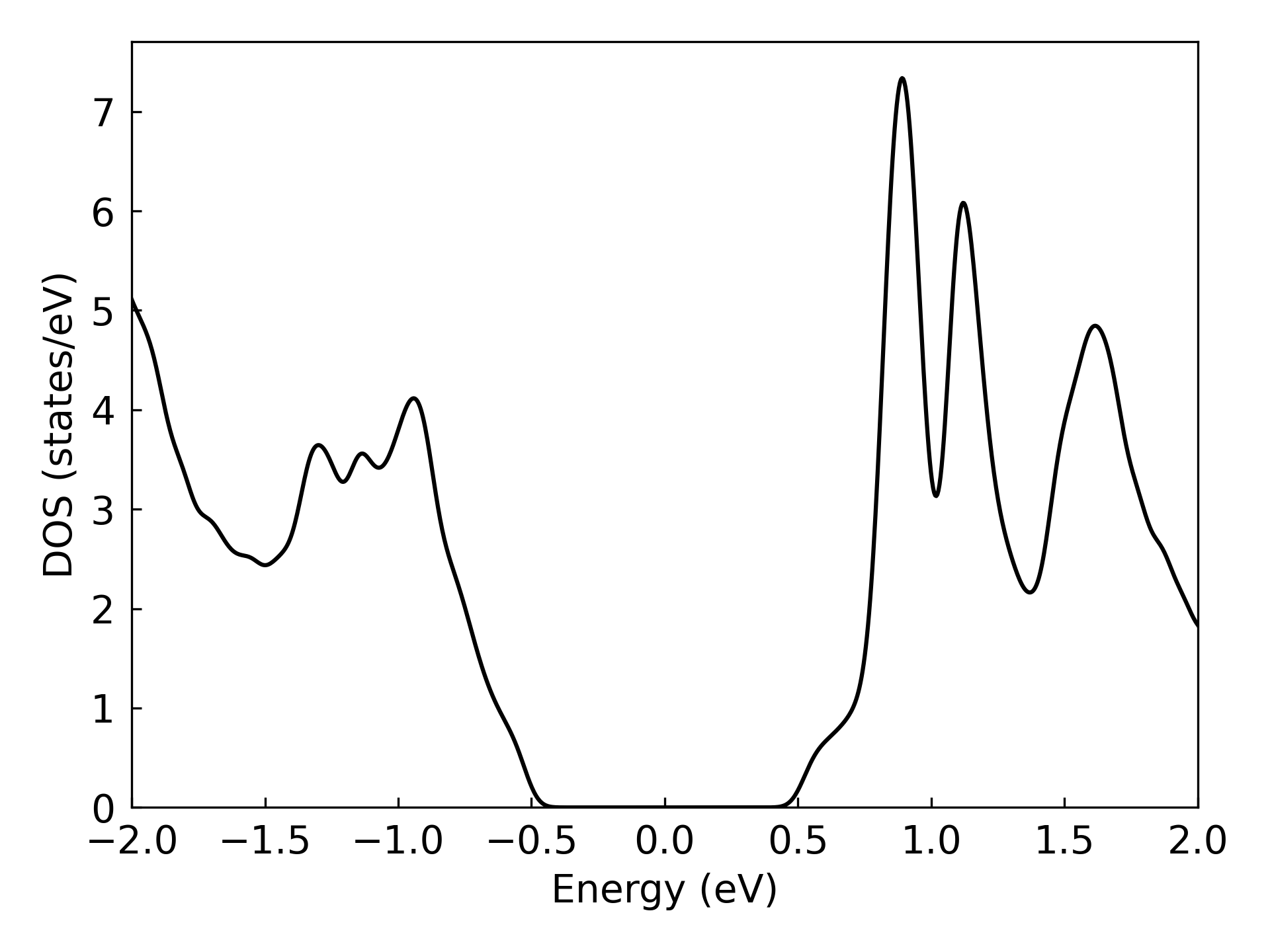
Density of states#
The energy eigenvalues output by find-fermi can be used to calculate the density of states (\(D_{(\varepsilon)}\)). The eigenvalues on a \(k\) mesh are discrete sampling points on the continuous energy bands, and should be expanded to give an approximation to the continuous \(D_{(\varepsilon)}\). The commonly used methods are smearing and tetrahedron method.
The density of states can be calculated by the following command:
dock compute eigen calc-dos -h
Usage: dock compute eigen calc-dos [OPTIONS] DATA_PATH

  Calc and plot the density of states.

Options:
  -j, --jobs-num INTEGER          Number of parallel workers. Default: -1 (auto-detect CPU cores).  [default: -1]
  --blas-parallel-mode            Use BLAS multi-threaded mode instead of parallel k-point mode (default).
  --method [gaussian|tetrahedron]
                                  Calculating method that is used for obtaining DOS.  [default: gaussian]
  -d, --kp-density FLOAT          The density of the k points.  [default: 0.1]
  --energy-window, --E-win <FLOAT FLOAT>...
                                  Plot band energy window (respect to fermi energy).  [default: -5, 5]
  -s, --smearing FLOAT            The smearing width (eV) in gaussian method.  [default: -1.0]
  --energy-num, --num INTEGER     Number of energy points.  [default: 201]
  --cache-res                     Cache the eigenvalues so that you can save time in the next same task.
  --ill-method [none|window|orbital]
                                  Method to handle ill-conditioned eigenvalues.  [default: none]
  --ill-threshold FLOAT           Threshold for ill-conditioned eigenvalue detection.  [default: 0.001]
  --window-emin FLOAT             Minimum energy for window regularization (eV, relative to Fermi).  [default: -1000.0]
  --window-emax FLOAT             Maximum energy for window regularization (eV, relative to Fermi).  [default: 6.0]
  -h, --help                      Show this message and exit.
The options jobs-num and --blas-parallel-mode control parallelization (see Fermi energy section for details). The cached result of eigenvalues will be used if its \(k\) mesh matches with current kp-density, otherwise the eigenvalues will be recalculated. The default expansion method is gaussian smearing, with -s option specifying the smearing width. The smearing width needs to be adjusted to balance between smoothness and fidelity of the plot. One can switch to the tetrahedron method by setting --method tetrahedron to perform more accurate calculation, and no parameters need to be adjusted.
Example:
dock compute eigen calc-dos ./eigen/MoTe2 -d 0.03 --energy-window -2.0 2.0 --energy-num 1000 -s 0.04 -j 16
Use cached fermi energy from fermi_energy.json
Use dk=0.03 and k_mesh=[58 58  1]
Calculating eigenvalues with k_mesh=[58 58  1], n_jobs=16 ...
Calculating DOS with emin=-2.0 eV, emax=2.0 eV, enum=1000, method=gaussian ...
  Using sigma=0.04 eV for gaussian smearing
Ploting DOS ...
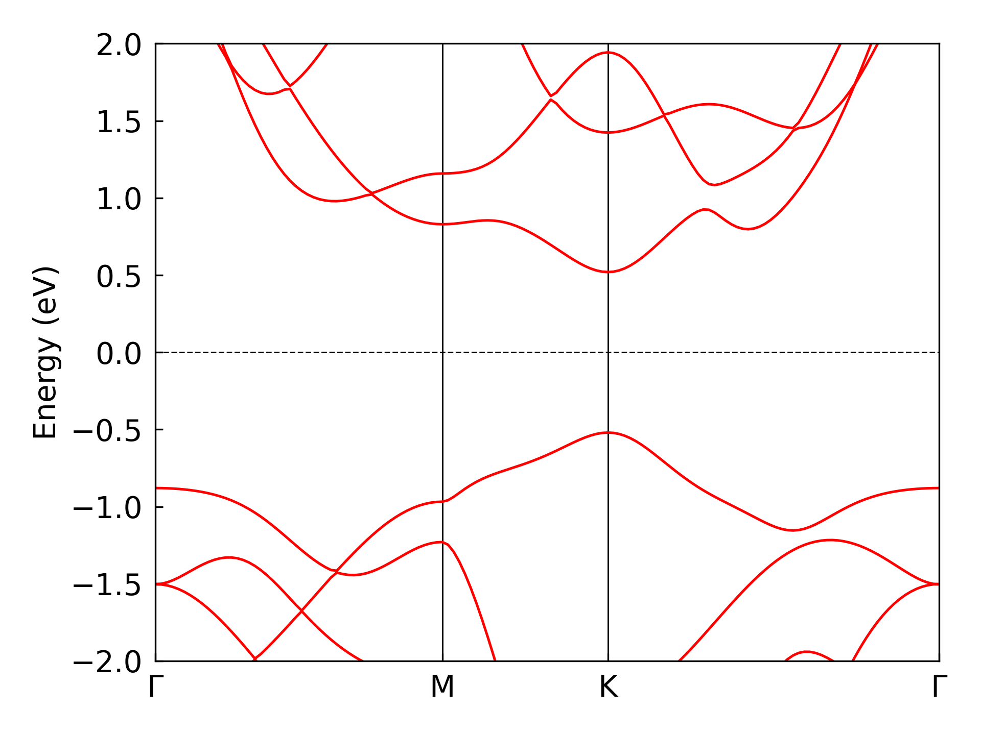
Band structure#
The band structure is one of the most basic and important electronic information in materials study. DeepH-dock provides terminal tool to calculate the band structure. The diagonalization is performed by the same module as previous sections, and the difference is that the \(k\) points are set along several paths in the reciprocal space.
The \(k\) paths need to be specified by the K_PATH file which looks like:
20  0.000000 0.000000 0.000000  0.000000 0.500000 0.000000  Gamma M
20  0.000000 0.500000 0.000000  0.333333 0.333333 0.000000  M K
20  0.333333 0.333333 0.000000  0.000000 0.000000 0.000000  K Gamma
In the K_PATH file, each row denotes a \(k\) path, with the first column specifying the number of \(k\) points in the path, and followed by the coordinates of the starting and ending \(k\) points in the reciprocal space. The last two columns specify the label of the starting and ending \(k\) points.
The band structure can be calculated by the following command. The calculation directory DATA_PATH should contain POSCAR, info.json, overlap.h5, hamiltonian.h5, and K_PATH.
dock compute eigen calc-band -h
Usage: dock compute eigen calc-band [OPTIONS] DATA_PATH

  Calculate the energy band and save it into h5 file.

Options:
  -j, --jobs-num INTEGER          Number of parallel workers. Default: -1 (auto-detect CPU cores).  [default: -1]
  --blas-parallel-mode            Use BLAS multi-threaded mode instead of parallel k-point mode (default).
  --sparse-calc                   Use sparse diagonalization.
  --num-band INTEGER              Number of bands when using sparse diagonalization.  [default: 50]
  --E-min, --min FLOAT            Lowest band energy (from the fermi level) when using sparse diagonalization.  [default: -0.5]
  --maxiter INTEGER               Max number of iterations when using sparse diagonalization.  [default: 300]
  --ill-method [none|window|orbital]
                              Method to handle ill-conditioned eigenvalues: 'none', 'window' (window regularization), or 'orbital' (orbital removal).  [default: none]
  --ill-threshold FLOAT       Threshold for ill-conditioned eigenvalue detection.  [default: 0.001]
  --window-emin FLOAT         Minimum energy for window regularization (eV, relative to Fermi).  [default: -1000.0]
  --window-emax FLOAT         Maximum energy for window regularization (eV, relative to Fermi).  [default: 6.0]
  -h, --help                  Show this message and exit.
The options jobs-num and --blas-parallel-mode control parallelization (see Fermi energy section for details). Sparse diagonalization is switched on by the --sparse_calc tag, and the options num-band, E-min and maxiter specify the behavior of the sparse solver.
Both the raw data band.h5 and the figure band.png is generated. The band.png is for a first glance and can be replotted by the following command:
dock compute eigen plot-band -h
Usage: dock compute eigen plot-band [OPTIONS] DATA_PATH

  Plot energy band with the h5 file that is calculated already.

Options:
  --energy-window, --E-win <FLOAT FLOAT>...
                                  Plot band energy window (respect to fermi energy).  [default: -5, 5]
  -h, --help                      Show this message and exit.
Example:
dock compute eigen calc-band ./eigen/MoTe2 -j 16
dock compute eigen plot-band ./eigen/MoTe2 --energy-window -2.0 2.0
Ill-Conditioned Eigenvalue Handling#
When using non-orthogonal basis sets, the overlap matrix \(S\) may have very small eigenvalues, causing the generalized eigenvalue problem \(H\psi = ES\psi\) to become numerically unstable. This produces “ill-conditioned eigenvalues” that are physically meaningless.
DeepH-dock provides two methods to handle ill-conditioned eigenvalues:
1. Window Regularization (--ill-method window)#
This method focuses on a specific energy window and projects out ill-conditioned eigenvalue components:
Solve the full generalized eigenvalue problem
Filter eigenvectors within the energy window \([E_{min}, E_{max}]\)
Construct quality matrix \(M = \Psi^\dagger \Psi\) to measure linear independence
Diagonalize \(M\) to find nearly linear-dependent combinations
Project onto well-conditioned subspace (\(\lambda_M > threshold\))
Re-solve in the reduced subspace
Best for: Band structure calculations where you care about specific energy ranges.
dock compute eigen calc-band ./data --ill-method window --ill-threshold 1e-3 --window-emin -5 --window-emax 5
2. Orbital Removal (--ill-method orbital)#
This method globally identifies and removes orbitals that cause ill-conditioning:
For each k-point, find the smallest eigenvalue of \(S(k)\) and its eigenvector
Find the k-point with globally smallest \(S\) eigenvalue
Identify the orbital with largest amplitude in that eigenvector
Remove that orbital from ALL k-points (maintains consistency)
Repeat until all \(S\) eigenvalues are above threshold
Best for: DOS calculations and when global orbital consistency is needed.
dock compute eigen calc-dos ./data --ill-method orbital --ill-threshold 5e-4
Comparison#
Feature |
Window Regularization |
Orbital Removal |
|---|---|---|
Removal Target |
Eigenvalue components |
Original orbital basis functions |
Approach |
Subspace projection |
Global orbital deletion |
Best Use |
Band structure, specific energy analysis |
DOS, global consistency |
Output Size |
Maintains original |
Reduced (removed slots filled) |
Parameters |
|
|
Class API#
DeepH-dock provides the HamiltonianObj class to deal with tight-binding Hamiltonian objects. Advanced users can construct the HamiltonianObj from the DeepH-pack format data and perform the operations (e.g., diagonalization, calculation of response properties and transition probabilities, etc.) by themselves.
from deepx_dock.compute.eigen.hamiltonian import HamiltonianObj
print(HamiltonianObj.__doc__)
from deepx_dock.compute.eigen.hamiltonian import HamiltonianObj
print(HamiltonianObj.diag.__doc__)
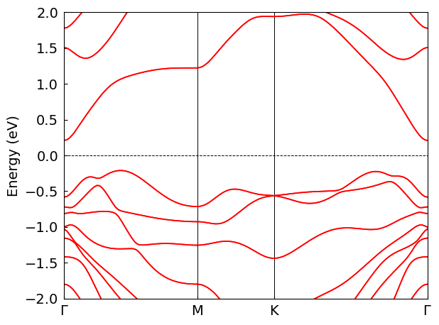
The example below shows how to construct the Hamiltonian operator and calculate the band structure.
from deepx_dock.compute.eigen.hamiltonian import HamiltonianObj
from deepx_dock.compute.eigen.band import BandDataGenerator, BandPlotter

data_path = "./eigen/Bi2Se3_SOC"
band_conf = {
    "k_list_spell" : """
        50   0.0000000000   0.0000000000   0.0000000000   0.5000000000   0.0000000000   0.0000000000     GAMMA               M
        30   0.5000000000   0.0000000000   0.0000000000   0.3333333333   0.3333333333   0.0000000000     M                   K
        60   0.3333333333   0.3333333333   0.0000000000   0.0000000000   0.0000000000   0.0000000000     K                   GAMMA
    """
}
band_data_path = "./eigen/Bi2Se3_SOC/band_data.h5"
window = [-2, 2]

obj_H = HamiltonianObj(data_path)
bd_gen = BandDataGenerator(obj_H, band_conf)
# Use parallel k-point mode with 4 workers (auto-detect: n_jobs=-1)
bd_gen.calc_band_data(n_jobs=-1, parallel_k=True)
bd_gen.dump_band_data(band_data_path)
bd_plotter = BandPlotter(band_data_path)
bd_plotter.plot(*window)
Using IllConditionedHandler in Python API#
For advanced control, you can use the IllConditionedHandler class directly:
from deepx_dock.compute.eigen.hamiltonian import HamiltonianObj
from deepx_dock.compute.eigen.ill_conditioned import IllConditionedHandler
import numpy as np

# Load Hamiltonian
data_path = "./eigen/Bi2Se3_SOC"
obj_H = HamiltonianObj(data_path)

# Define k-points
ks = np.array([[0.0, 0.0, 0.0], [0.5, 0.0, 0.0], [0.5, 0.5, 0.0]])

# Method 1: Window Regularization
print("=== Window Regularization ===")
ill_handler_window = IllConditionedHandler(
    method='window_regularization',
    ill_threshold=1e-3,
    window_emin=-5.0,   # relative to Fermi energy
    window_emax=5.0,
    fermi_energy=obj_H.fermi_energy,
)
eigvals_window = obj_H.diag(ks, n_jobs=-1, parallel_k=True, ill_handler=ill_handler_window)
print(f"Eigenvalues shape: {eigvals_window.shape}")
print(f"Min eigenvalue: {eigvals_window.min():.4f} eV")

# Method 2: Orbital Removal
print("\n=== Orbital Removal ===")
ill_handler_orbital = IllConditionedHandler(
    method='orbital_removal',
    ill_threshold=5e-4,
)

# For orbital removal, first get all overlap matrices
Sk_list = obj_H.get_all_Sk(ks, n_jobs=-1, parallel_k=True)
ill_handler_orbital.prepare_orbital_truncation(Sk_list)
print(f"Kept orbitals: {len(ill_handler_orbital.kept_orbitals)}/{obj_H.orbits_quantity}")

eigvals_orbital = obj_H.diag(ks, n_jobs=-1, parallel_k=True, ill_handler=ill_handler_orbital)
print(f"Eigenvalues shape: {eigvals_orbital.shape}")
print(f"Min eigenvalue: {eigvals_orbital.min():.4f} eV")
=== Window Regularization ===
Eigenvalues shape: (160, 3)
Min eigenvalue: -21.8541 eV

=== Orbital Removal ===
[done] Kept 160/160 orbitals
Kept orbitals: 160/80
Eigenvalues shape: (160, 3)
Min eigenvalue: -21.8541 eV
# Get information about the handler configuration
print(ill_handler_window.get_info())
{'method': 'window_regularization', 'ill_threshold': 0.001, 'window_emin': -2.6445907560210653, 'window_emax': 7.355409243978935, 'fill_value': 10000.0}
Low-Level Functions#
You can also use the low-level functions directly for fine-grained control:
from deepx_dock.compute.eigen.ill_conditioned import (
    window_regularization_eig,
    global_orbital_truncation,
    eig_with_orbital_mask
)

# Get H(k) and S(k) for a single k-point
k = np.array([0.0, 0.0, 0.0])
Sk, Hk = obj_H.Sk_and_Hk(k)

# Apply window regularization directly
eigvals_wr, eigvecs_wr = window_regularization_eig(
    Hk, Sk,
    emin=obj_H.fermi_energy - 5.0,
    emax=obj_H.fermi_energy + 5.0,
    ill_threshold=1e-3,
    return_vecs=True
)
print(f"Window regularization: {eigvals_wr.shape}")

# Get multiple k-points for orbital truncation
ks_mesh = np.array([[i/10, j/10, 0.0] for i in range(3) for j in range(3)])
Sk_list = [obj_H.Sk_and_Hk(k)[0] for k in ks_mesh]

# Find orbitals to keep
kept_orbitals = global_orbital_truncation(Sk_list, ill_threshold=5e-4, verbose=True)

# Apply orbital mask directly
eigvals_om, eigvecs_om = eig_with_orbital_mask(
    Hk, Sk, kept_orbitals,
    return_vecs=True
)
print(f"Orbital mask: {eigvals_om.shape}")
Window regularization: (160,)
[done] Kept 160/160 orbitals
Orbital mask: (160,)