Making Prediction#
In this part, we demonstrate some quick examples for DeepH inference. The ability of electronic structure inference on ultra-large systems is the very purpose of DeepH-pack. After training on small systems with relatively small computation amount, the neural-network models can generalize to larger systems with both high accuracy and efficiency.
Prepare the Dataset for Inference#
In the inference process, the hamiltonian matrix is not pre-known and the overlap matrix is a necessary input. The sparsity pattern of the overlap matrix is indispensable for constructing the atomic connectivity graph during inference. The data required by the inference process are listed as follows, and the key point is obtaining the overlap matrix.
dft
  |- 0
     |- POSCAR
     |- info.json
     |- overlap.h5
  |- 1
  |- ...
NOTE:
Although the specific values of overlap matrix do not affect the behavior of the neural network model, the actual numerical values become essential for post-processes such as diagonalization for obtaining band structures. In other words, the calculation of overlap matrix is always needed for the complete workflow.
In most of the ab initio programs based on localized orbitals, the overlap matrix can be efficiently calculated by a single non-self-consistent calculation without executing costly SCF cycles or matrix diagonalization. So that the overlap generation process does not affect the overall \(O(N)\) time-cost of the inference workflow of DeepH-pack.
Using DeepH-dock to Obtain the Overlap Matrix#
DeepH-dock, in conjunction with HPRO, provides a direct and recommended approach for calculating overlap matrix elements of arbitrary materials, given the required basis set files. This integrated method is favored over alternative workflows that involve subsequent code modifications. Currently, DeepH-dock only supports computation of overlap matrices from SIESTA basis files, but support for more DFT data formats will come out soon.
Overlap computation: FHI-aims#
By setting sc_iter_limit = 0 in FHI-aims, users can perform a single-step non-self-consistent calculation that extracts the overlap matrix, while maintaining the fundamental capability that DeepH inference itself requires only POSCAR and info.json to predict Hamiltonians – with DFT-level computations remaining strictly optional for result verification.
Overlap computation: SIESTA#
By setting MaxSCFIterations as 0 in SIESTA, users can perform a single-step non-self-consistent calculation that extracts the overlap matrix.
Overlap computation: OpenMX#
There is no built-in option to perform an overlap-only calculation by OpenMX, so that one needs to modify the OpenMX source code. Please refer to the overlap-only-OpenMX repository for details. This modified verson of OpenMX will exit after dumping the overlap-matrix. Then the dumped overlap matrix (in the old data format of DeepH) can be converted to the new data format by DeepH-dock.
Overlap computation: ABACUS#
To perform an overlap-only calculation by ABACUS, calculation get_S should be specified in the INPUT file instead of calculation scf, and no further modification of the source code is needed. The program will exit after dumping the SR.csr file, and it can be converted to the new data format by DeepH-dock.
Inference with DeepH#
The inference process can be performed on CPU or GPU platforms. Although GPU platform is much faster, the memory (e.g., 24GB for NVIDIA 4090 GPUs) is not enough for large systems (e.g., 10000 atoms in the unitcell). So that CPU platform is more commonly used for inference.
The inference setup contains three essential components:
TOML configuration file
inputs/directory (containing the POSCAR, info.json, and overlap.h5)model/directory (containing the optimized model parameters)
FHI-aims \(\text{H}_2\text{O}\)#
For the \(\text{H}_2\text{O}\) system we just trained in the previous chapter, we can use the following configuration file for inference.
The ./inputs/dft directory is already linked to the dataset used for training.
# ---------------------------------- SYSTEM ----------------------------------
[system]
note = "Enjoy DeepH-pack! ;-)"
device = "gpu*1"
float_type = "fp32"
random_seed = 137
log_level = "info"
jax_memory_preallocate = true


# ----------------------------------- DATA ------------------------------------
[data]
inputs_dir = "./inputs"
outputs_dir = "./outputs"

[data.dft]
data_dir_depth = 0
validation_check = false

[data.graph]
dataset_name = "H2O_5K_FHI-aims"
graph_type = "S"
storage_type = "memory"
parallel_num = -1
only_save_graph = false


# ----------------------------- MODEL -----------------------------------------
[model]
model_dir = "../../4.Training/H2O_5K_FHI-aims/outputs/2025-10-14_10-34-43/model"
load_model_type = "best"
load_model_epoch = -1


# ------------------------------ PROCESS --------------------------------------
[process.infer]
output_type = "h5"
output_into = "to_output"
target_symmetrize = true
multi_way_jit_num = 1

[process.infer.dataloader]
batch_size = 1000
NOTE:
The
model.model_diris the directory where the model is saved during training, both the relative and absolute path are supported. The directory should end with “model”. Themodel.load_model_typeselects the “latest.pytree” or “best.pytree” under the model_dir.The
process.infer.output_intocontrols the location of the output hamiltonians, “to_output” fordata.outputs_dir.dftand “to_input” fordata.inputs_dir.dft.
To execute the inference process on the supercomputing platforms with job management system like slurm, it is recommend to write a script and then submit the inference job.
#!/bin/bash
#
#SBATCH --job-name=H2O-infer
#SBATCH --gpus=1
#SBATCH -p vip_gpu_sczc641

module load cuda/12.9
source ~/.uvenv/deeph/bin/activate

deeph-infer infer.toml
The configuration file and submit script are already placed under the “H2O_5K_FHI-aims” folder, and one can execute the inference process by one command:
sbatch submit.sh
The inference results will subsequently be written to the outputs (or inputs) directory as hamiltonian_pred.h5.
infer-outputs/<timestamp>
  |- deepx.log
  |- dft
    |- 0
       |- hamiltonian_pred.h5
    |- 1
       |- hamiltonian_pred.h5
    |- ...
The water-related training and inference examples provided earlier serve primarily as simplified demonstrations to showcase DeepH’s potential in realistic scientific applications.
These examples demonstrate DeepH’s capability to transform massive quantum material datasets into compact, high-precision computational models. Both the sparrow and eagle net perform well on the datasets generated by a variety of DFT softwares. The sparrow net acheives high accuracy with low computation overhead, and the eagle net acheives even higher accuracy (50% to 100% improvement upon sparrow net) with an acceptable trade-off in efficiency (approximately 50% slower than sparrow net). This allows users to select the most suitable network settings based on their specific purposes.
Error Analysis#
For detailed instructions, see DeepH-pack: Analyze Error.
To confirm the validity of the model, the inference result hamiltonian_pred.h5 is compared with the benchmark data hamiltonian.h5. The error extraction and visualization can be done by the dock analyze error command in DeepH-dock. It gives detailed error distribution, not just a loss value.
cd ./outputs/<timestamp>
dock analyze error structure ./dft -b ../../inputs/dft -p 4 --cache-res
This will generate a figure error_structure_distribution.png showing the error distribution of each structure. The result of the \(\text{MoS}_2\) example is shown below:
cd ./outputs/<timestamp>
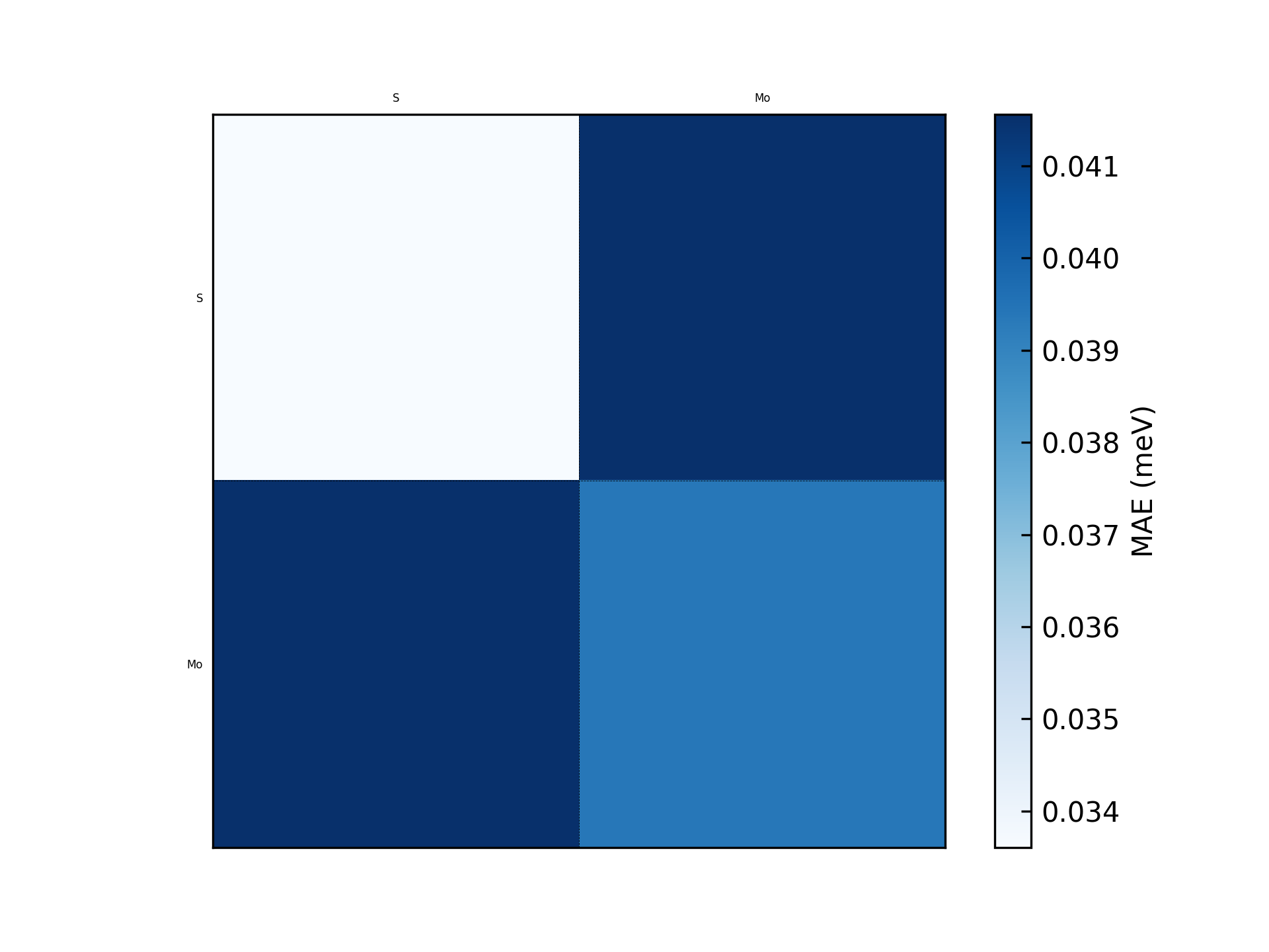
dock.error.ExposeErrorDist dft -b ../../inputs/dft -k orbital -p 5
This will generate a figure error_orbital_resolute_distribution.png showing the error decomposed on each orbital-pair. The result of the \(\text{MoS}_2\) example is shown below:
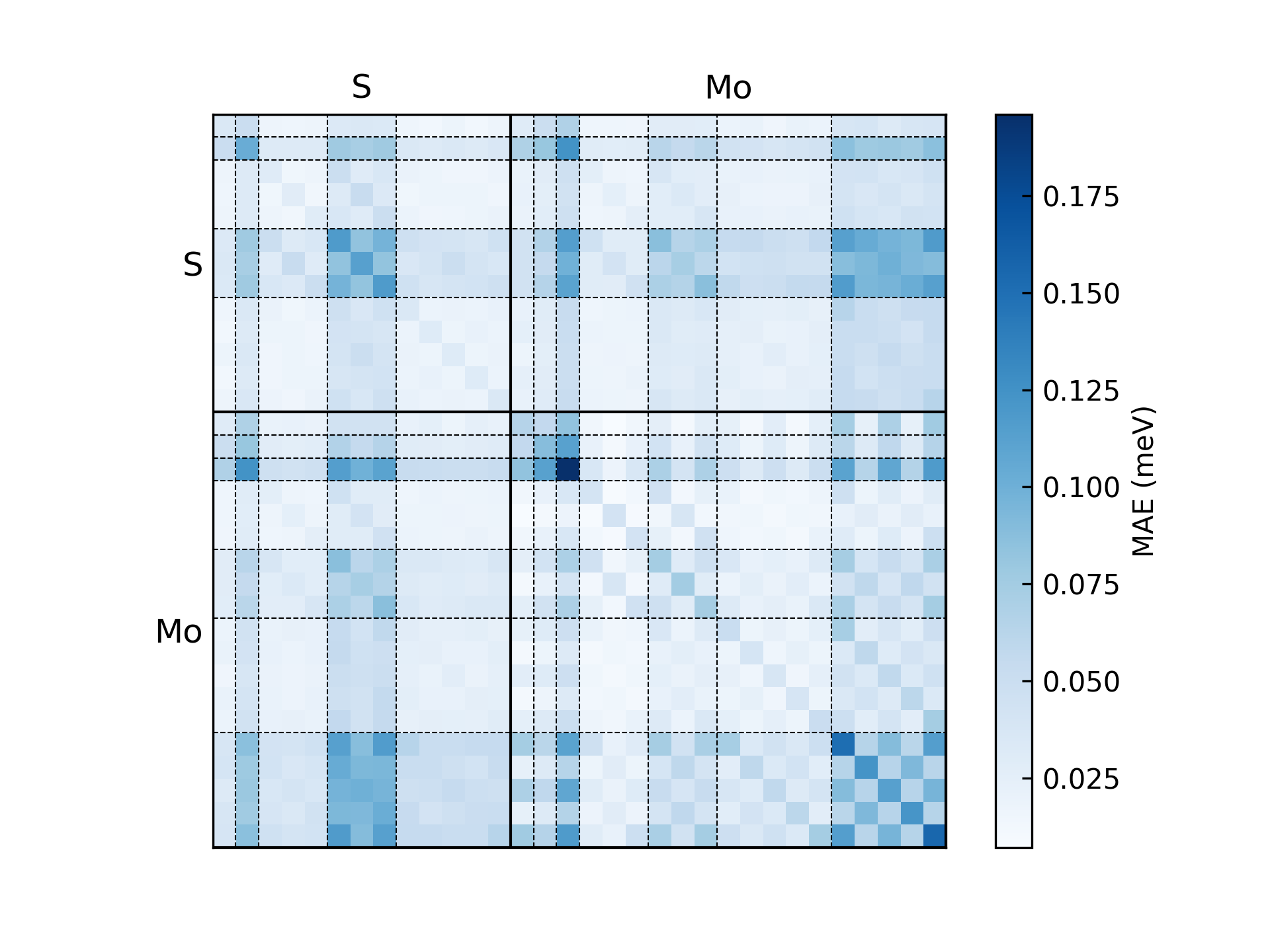
Several error modes are available:
orbital: error for each orbital pair.element-pair: error for each element pair.element(-logfile): error of each element.entries: error for matrix entries with scatter figure.structure(-logfile): error distribution of each structure.
NOTE:
The raw data (not just the figure) can be dumped by
--cache_resoption.Use
--data_split_jsonand related options to select a subset for error statistics.
Determine and update the Fermi energy#
For detailed instructions, see DeepH-pack: Compute Hamiltonian Diagonalization.
After obtaining the predicted Hamiltonian (by default named as hamiltonian_pred.h5) through the inferencing process, you can diagonalize it and plot the corresponding band structures with the help of DeepH-dock, facilitating subsequent analysis and comparison.
In DeepH, Hamiltonians differing only by an energy shift gauge transformation (\(H' = H - \mu S\)) are considered equivalent. DeepH predictions do not guarantee gauge invariance, particularly when training datasets contain structures with significantly divergent gauge choices. Under such conditions, re-evaluating the Fermi energy based on electron occupation numbers becomes essential. The deeph-dock toolkit provides specialized utilities for this purpose. Users must first prepare the following four prerequisite files:
cd MoS2_500_OpenMX/band/502
ln -s ../../outputs/<timestamp>/dft/502/hamiltonian_pred.h5 ./hamiltonian.h5
Where the <timestamp> is your inference time_stamp. The current directory looks like below:
band/502/
    |- POSCAR
    |- info.json
    |- overlap.h5
    |- hamiltonian.h5 -> ../../outputs/<timestamp>/dft/502/hamiltonian_pred.h5
Subsequently, the total valence electron count must be provided under the “occupation” key in info.json. It is usually included in the output file of the program, otherwise it can be calculated using the pesudo-potential information. Take \(\text{Mo}_{25}\text{S}_{50}\) for example, for OpenMX with PBE19 pesudopotential, the occupation is the sum of the valence electrons, i.e., \(14\times 25 + 6\times 50=650\), and for FHI-aims which is an all-electron program, the occupation is the sum of the atomic numbers, i.e., precisely \(42\times 25 + 16\times 50 = 1,850\).
{
    "occupation": 650, # OpenMX with PBE19 pesudopotential
    "atoms_quantity": 75,
    "orbits_quantity": 1125,
    "orthogonal_basis": false,
    "spinful": false,
    "fermi_energy_eV": 0.0,
    "elements_orbital_map": {"Mo": [0, 0, 0, 1, 1, 2, 2], "S": [0, 0, 1, 1, 2]}
}
NOTE: The occupation here always includes spin degeneracy, and the program automatically deals with the spin-degeneracy when spinful is false. For the spinless case above, it will give \(650\div 2 = 325\) occupied bands.
Subsequently, simply execute the following command within the data directory to compute the Fermi energy.
cd band/502
dock compute eigen find-fermi ./ -p 5
The calculated Fermi energy will be stored in fermi_energy.json.
{"fermi_energy_eV": -4.966581910156199}
Use this value to repalace the “fermi_energy_eV” in info.json and you are ready to run the band structure calculation.
NOTE: Users may notice that automatic Fermi level updating is intentionally unavailable in this implementation. This design choice stems from two core principles:
Preserving raw data integrity is paramount in neural network training, as modifying source datasets carries inherent risks – we therefore implement deliberate barriers against accidental misuse.
We encourage users to implement simple functionalities through Python scripting, analogous to creating Bash scripts for data extraction. DeepH-pack prioritizes providing a flexible computational framework over delivering an all-in-one black-box program.
Plotting the band structure#
In order to obtain the band structures, an additional file K_PATH is required during the band structure calculation. This file specifies the high-symmetry path for the band structure and can be written manually. For layered \(\text{MoS}_2\) the path can be:
20  0.000000 0.000000 0.000000  0.000000 0.500000 0.000000  Gamma M
20  0.000000 0.500000 0.000000  0.333333 0.333333 0.000000  M K
20  0.333333 0.333333 0.000000  0.000000 0.000000 0.000000  K Gamma
With each line contains: k-point count, fractional coordinates of the first and second high-symmetry points, followed by their labels.
band/502/
    |- POSCAR
    |- info.json
    |- overlap.h5
    |- hamiltonian.h5 -> ../../outputs/<timestamp>/dft/502/hamiltonian_pred.h5
    |- K_PATH
Finally, you can use the following command to obtain the band structure plot:
cd band/502
dock compute eigen calc-band ./ -p 5
The -p 5 specifies 5-core parallelization over k points and can be adjusted according to available computational resources.
After obtaining the band file band.h5, you can plot the band structure with the following command:
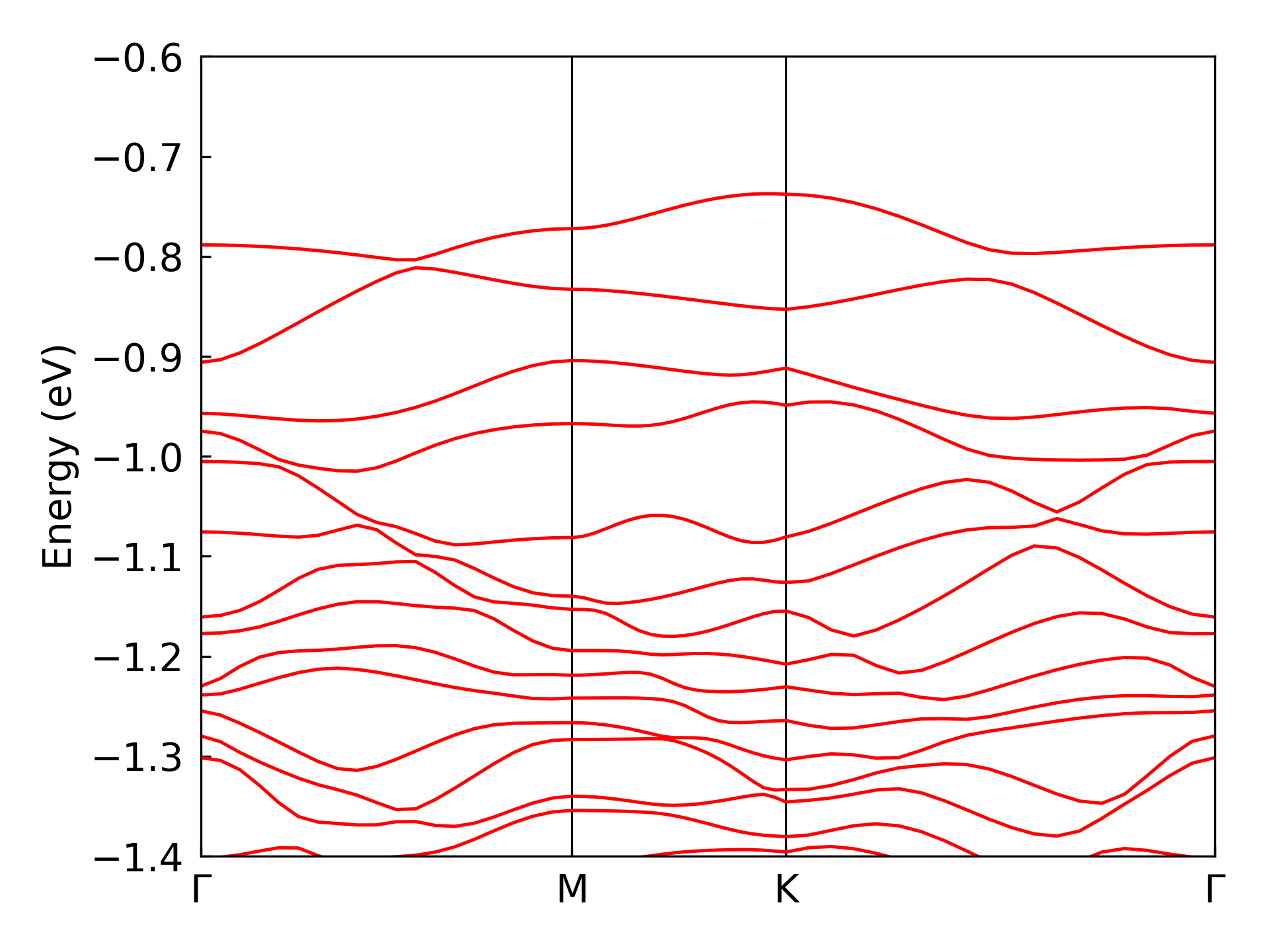
dock compute eigen plot-band ./ --energy-window <Emin> <Emax>
where --energy-window set the energy bounds for the band structure plot. The obtained band structure plot is shown in the figure below:
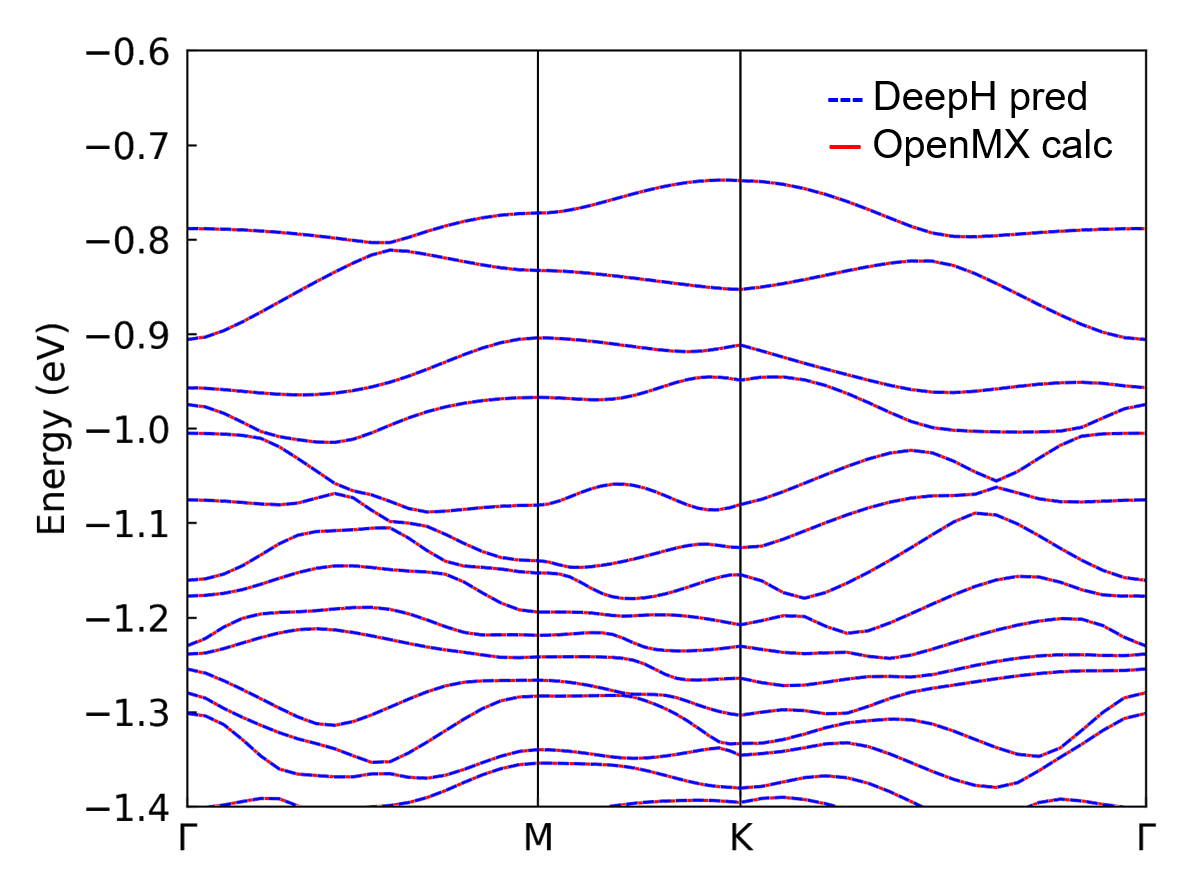
Comparision with benchmark data#
If the data calculated by the first-principle softwares is available, the band structure from the first-principle calculation and DeepH-pack inference can be combined together for comparison. The comparison plot of a \(\text{MoS}_2\) structure is shown below:
DeepH-Accelerated Self-Consistent Calculations#
As demonstrated above, the Hamiltonians predicted by DeepH are significantly superior to the initial guess Hamiltonians inside the ab-initio softwares. By feeding DeepH-predicted Hamiltonians back into the software as restart guesses for continued calculations, the number of SCF iteration steps required for convergence can be dramatically reduced. The corresponding data pipeline is currently under development and will soon be released in the deeph-dock toolkit.