
Basic Usage#
AimsPy is primarily used through its Python API, with a small command-line interface for managing the bundled FHI-aims patch. This page walks through the common workflows.
Note: Forward SCF calculations work with any system type. However, extracting or injecting matrices (Hamiltonian, overlap, H_init, which are used in warmstart, capture, and export workflows below) requires a periodic system with
use_local_index = .false.. For isolated molecules, use a sufficiently large periodic cell with vacuum (see thefrom_scratch/run.pyexample).
1. Python API#
Baseline SCF#
The most common entry point is the one-shot Calculator.do() (or Calculator.init() then Calculator.calc()) wrapped in a context manager:
from mpi4py import MPI
from aimspy import Calculator, CalculatorConfig

comm = MPI.COMM_WORLD
rank = comm.rank

config = CalculatorConfig(lib_path="/path/to/libaims.so")
with Calculator(config) as calc:
    calc.do(comm=comm, work_dir="./MoS2")
    if rank == 0:
        H = calc.hamiltonian     # AimspyMatrix (block-sparse, Hartree, rank-0 only)
        S = calc.overlap         # rank-0 fallback (see capture_overlap below)
    E = calc.energy          # float (Hartree)
    F = calc.forces          # (n_atoms, 3) ndarray in eV/Å, or None
Run with MPI:
mpiexec -np 8 python run_aims.py
work_dir must contain control.in + geometry.in, just like in a standard FHI-aims calculation.
Because of the multiple processes involved with MPI, the Calculator not thread-safe.
Export to DeepH format#
Export converged Hamiltonian, overlap, and free-atom initial Hamiltonian to the DeepH on-disk format:
from mpi4py import MPI
from aimspy import Calculator, CalculatorConfig
from aimspy import DeepHData

comm = MPI.COMM_WORLD
rank = comm.rank

config = CalculatorConfig(
    lib_path="/path/to/libaims.so",
    capture_initial_hamiltonian=True,  # capture free-atom H0
)
with Calculator(config) as calc:
    calc.do(comm=comm, work_dir="./MoS2")

    # Export H, S, H0 to DeepH on-disk format
    if rank == 0:
        dd = DeepHData.from_aimspy(
            calc.structure,
            hamiltonian=calc.hamiltonian,
            overlap=calc.overlap,
            initial_hamiltonian=calc.initial_hamiltonian,
        )
        dd.save("deeph_out/")
To additionally export force-field labels to force.h5, pass the available
energy, force, and stress observables:
    if rank == 0:
        dd = DeepHData.from_aimspy(
            calc.structure,
            hamiltonian=calc.hamiltonian,
            overlap=calc.overlap,
            initial_hamiltonian=calc.initial_hamiltonian,
            force=calc.forces,    # (n_atoms, 3) eV/Å, aims order — auto-reordered to POSCAR
            energy=calc.energy_free_relative,  # Hartree — auto-converted to eV
            stress=calc.stress,   # (3, 3) eV/ų
        )
        dd.save("deeph_out/")    # writes force.h5 alongside H/S/H0
Energy and force are optional and omitted when unavailable. Stress is always
written when force.h5 is created: if calc.stress is None, the (6,)
dataset contains zeros in [xx, yy, zz, yz, xz, xy] order. calc.forces
requires compute_forces .true. and nonzero analytical stress data requires
compute_analytical_stress .true. in control.in.
calc.energy_free_relative is the force-consistent electronic free energy
minus the sum of the radial free-atom reference energies that FHI-aims already
computes for the resolved species settings. Use
calc.free_atom_reference_energies for the per-species values and
calc.free_atom_reference_energy for their composition-weighted sum.
Note: For the DeepH on-disk data format specification (POSCAR, info.json, .h5 files), see DeepH-dock Key Concepts.
DeepH warmstart#
The central use case for AimsPy. Inject a pre-trained DeepH Hamiltonian as the initial guess and converge SCF in several iterations:
from mpi4py import MPI
from aimspy import Calculator, CalculatorConfig, Strategy
from aimspy import DeepHData

data = DeepHData.from_directory("deeph_out/")
config = CalculatorConfig(lib_path="/path/to/libaims.so")
calc = Calculator(config)
calc.modify_init_ham(source=data, strategy=Strategy.REPLACE)
calc.do(comm=MPI.COMM_WORLD, work_dir="./MoS2")
Deferred source
generate the source at runtime (after H_init/overlap are available, inside the python_func callback):
config = CalculatorConfig(
    lib_path="/path/to/libaims.so",
    capture_initial_hamiltonian=True,
    capture_overlap=True,
)
calc = Calculator(config)

@calc.modify_init_ham(strategy=Strategy.REPLACE, option={"deeph_path": "deeph_out/"})
def gen_source(calculator, option):
    # calculator.initial_hamiltonian / .overlap available here
    return DeepHData.from_directory(option["deeph_path"])

calc.do(comm=MPI.COMM_WORLD, work_dir="./MoS2")
Modification strategies#
The Strategy enum covers the common H0-modification cases:
Strategy |
Behaviour |
Required argument |
|---|---|---|
|
Clear and copy the external Hamiltonian’s blocks into the live H0 (H_init) buffer |
|
|
Add external blocks on top of the live H0 (e.g. a predicted H − H₀ to recover H) |
|
|
Multiply the live H0 by a constant factor |
|
|
Call |
|
For technical details on each strategy and the modify_init_ham API (direct vs. deferred mode, state guards), see Key Concepts.
Capturing overlap and the free-atom H0#
Two CalculatorConfig flags opt in to additional callbacks:
config = CalculatorConfig(
    lib_path="/path/to/libaims.so",
    capture_initial_hamiltonian=True,   # export_h0 callback
    capture_overlap=True,               # export_ovlp callback (live, all ranks)
)
with Calculator(config) as calc:
    calc.do(comm=MPI.COMM_WORLD, work_dir="./MoS2")
    H0 = calc.initial_hamiltonian        # free-atom H_init (AimspyMatrix)
    S  = calc.overlap                    # live overlap on all ranks
Without capture_overlap, calc.overlap falls back to a rank-0 snapshot taken after calc().
Real-space grid data capture#
Capture the converged electron density, Kohn-Sham potential, and grid geometry for post-processing:
from mpi4py import MPI
from aimspy import Calculator, CalculatorConfig

comm = MPI.COMM_WORLD
rank = comm.rank

config = CalculatorConfig(
    lib_path="/path/to/libaims.so",
    capture_grid_data=True,  # export_grid_data callback
)
with Calculator(config) as calc:
    calc.do(comm=comm, work_dir="./MoS2")
    if rank == 0:
        gd = calc.grid_data              # GridData object
        gd.save_npz("grid.npz")          # save for offline analysis

        # Derived quantities
        print(f"delta_rho: {gd.delta_rho.min():.3e} .. {gd.delta_rho.max():.3e}")
        print(f"vxc range: {gd.vxc.min():.3f} .. {gd.vxc.max():.3f} Ha")
GridData fields include coords, rho, vks, vks0, vh, vh0, rho0, and structure fields (atom_coords, atom_symbols, lattice). See Key Concepts for the full field reference and units.
MPI gather: GridData.gather(local, comm) collects per-rank subsets to root using Gatherv (memory-efficient, zero-pickle). Root peak memory is ~1x the total dataset vs ~3x for pickle-based gather.
Visualization: the aimspy.viz module provides plotting helpers:
from aimspy import viz

viz.scatter_slice(gd, value="delta_rho", ax=ax)  # 2-D scatter slice
viz.radial_profile(gd, value="rho", atom_index=0)  # radial profile
viz requires matplotlib (imported lazily). 3-D isosurfaces require pyvista (optional).
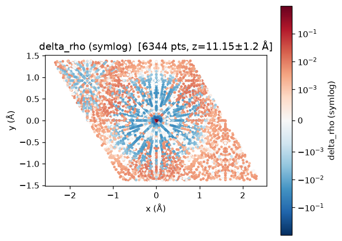
Example: viz.scatter_slice(gd, value="delta_rho") on MoS₂ (LDA). The
symlog colour scale reveals weak charge-transfer features (0.001–0.01
e/bohr³) that a linear scale would flatten.
NAO radial basis capture#
Capture the complete cubic-spline representation of the NAO radial basis
functions (u(r), (e−v)·u(r), du/dr, plus per-species log-grid parameters).
The callback fires once inside prepare_scf — before any SCF iteration —
so the data is available right after calc.init() (no calc() needed):
config = CalculatorConfig(
    lib_path="/path/to/libaims.so",
    capture_basis_data=True,  # export_basis_data callback (registered pre-init)
)
with Calculator(config) as calc:
    calc.do(comm=comm, work_dir="./MoS2")
    if rank == 0:
        bd = calc.basis_data            # BasisData object

        # Evaluate radial functions at arbitrary distances (bohr)
        u = bd.evaluate_u(0, [0.5, 1.0, 2.0])   # species map attached automatically

        # Incremental H5 library (existing elements are skipped, not
        # overwritten), then plot offline:
        bd.save_h5("basis.h5", calc.info)
aimspy viz-basis basis.h5 -o figures/ # one radial-basis figure per element
See Key Concepts for the
basis.h5 layout, evaluation semantics, and units.
Error recovery#
If SCF crashes, use force_close() (always safe) and create a fresh Calculator.
FHI-aims is a global singleton: one init/finalize cycle per process, so a finalized Calculator cannot be reused.
Note:
close()/force_close()now callsaimspy_export_grid_data_finalize()to explicitly deallocate Fortran-side grid buffers (coords, potentials, vdW), preventing ~500 MB memory retention after the Calculator is closed.
Context manager (recommended: __exit__ auto-calls force_close() on exception):
config = CalculatorConfig(lib_path="...")
try:
    with Calculator(config) as calc:
        calc.do(comm=MPI.COMM_WORLD, work_dir="./MoS2")
        H = calc.hamiltonian
except Exception as e:
    print(f"SCF failed: {e}")
    # Calculator already force_closed by __exit__; create a new one to retry
Manual pattern (when you need finer control):
calc = Calculator(CalculatorConfig(lib_path="..."))
try:
    calc.do(comm=MPI.COMM_WORLD, work_dir="./bad_input")
except Exception:
    calc.force_close()
    # create a new Calculator for the next run
close() is the graceful counterpart, silent no-op from UNINIT/FINALIZED, raises AimspyStateError from RUNNING (use force_close), and a normal finalize from INITED/DONE.
2. Command-line Tool#
The aimspy CLI provides patch (manage the bundled FHI-aims patch: apply, uninstall, dry-run, list) and the visualization front-ends viz-basis / viz-grid (offline plotting from basis.h5 / grid npz files). See the CLI reference for full options and examples.
3. Learning Through Examples#
The examples/ directory in the repository contains two runnable end-to-end scripts:
from_scratch/run.pyH₂O baseline SCF + DeepH export. DemonstratesCalculatorConfig.capture_initial_hamiltonian=True+capture_overlap=True, andDeepHData.from_aimspy(...).save(...).continue_calc/run.pywarmstart demo. Loads the previous run’s DeepH output viaDeepHData.from_directory, appliesStrategy.REPLACEviamodify_init_ham(source=data), and shows SCF converging in several iterations.
Run them with:
export AIMSPY_TEST_AIMS_LIBPATH=/path/to/libaims.so
make run-from-scratch
make run-continue-calc    # requires run-from-scratch first
A MoS₂ integration test fixture (including a reference rs_hamiltonian.out) is available under tests/data/MoS2/ for cross-validation.
4. Extending AimsPy#
AimsPy is designed with extensibility in mind. If you want to add new functionality:
New external matrix source implement the
ExternalMatrixSourceprotocol in a new subpackage underaimspy/interface/<your_format>/.New callback follow the extension contract documented in the Development Guide.
New modification strategy extend the
Strategyenum and the_apply_strategydispatcher.
For detailed guidance, refer to the Development Guide.
Need Help?#
Use
aimspy patch --helpfor CLI assistance.Check the
examples/directory for practical implementations.For technical background on the in-memory architecture, callbacks, and data formats, see Key Concepts.
For development questions, see the For Developers section.